In the previous blog post, we looked at the basics of running R procedures in SPSS syntax. In this post, we’re going to explore how to work with R packages. Packages are collections of functions and pre-built compiled code that enable R users to carry out a vast range of analytical and data manipulation tasks. In fact, there are more than 10,000 user contributed packages available to the R user community and this number is growing all the time. Moreover, any R installation already includes a set of base packages which are regarded as part of the R source code. The directories in R where the packages are stored are called the libraries. You should bear in mind that the term library is often used as if it was synonymous with package, even though technically speaking they are separate things. You can actually view which packages are loaded in your current R session within SPSS, using the following code snippet.
BEGIN PROGRAM R.
sessionInfo()
END PROGRAM.
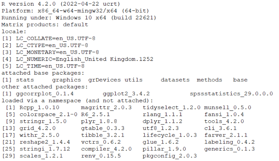
Here are the results of running this procedure during my own SPSS and R session.
In this post, we will see how to install and work with an R package that allows us to generate colourful correlograms within SPSS. The package we’ve chosen to work with is called ggcorrplotand it allows us to visualise a correlation matrix using colour coding to represent the magnitude of the correlation coefficients. To install a new package in R, we need only use the install.packages(“”)command. The package can then be called for use in a session using the library()command. It’s also worth noting that package names are case sensitive. The first part of following code snippet downloads and installs the package ggcorrplot. Once installed, we wouldn’t normally need to install it again, although if a new version is released, we may wish to update it. The second procedure then simply loads the package for use during a session.
BEGIN PROGRAM R.
install.packages("ggcorrplot")
library (ggcorrplot)
END PROGRAM.
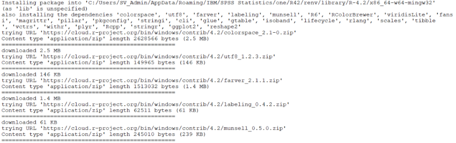
Executing the install.packages(“”)command causes R to immediately connect to its default online resource (https://cloud.r-project.org) and begin downloading the required package. You should see some system information regarding this process in the log file output in the SPSS Viewer window.
Once the package is installed, the library (ggcorrplot)command calls the package and loads it into the memory space of the current session.
At this point, we can take a closer look at how the ggcorrplot package is applied to data and the various ways in which we can control the output it produces.
In our example, we will build the correlogram from a matrix of correlation coefficients. To do this, we will use the cor function in R which allows us to compute correlation, variance and covariance matrices. Note: it also possible to compute a matrix of correlation p values using the cor_pmat function.
To introduce this, look at the following block of R code.
BEGIN PROGRAM R.
#install.packages("ggcorrplot")
library (ggcorrplot)
df_SPSS <- spssdata.GetDataFromSPSS()
df_CORR <- df_SPSS[c('salbegin','salary','age','educ','prevexp')]
CORRmat <- round(cor(df_CORR,  use = "pairwise.complete.obs", ),2)
head(CORRmat)
ggcorrplot(CORRmat)
END PROGRAM.
After using the library()command to call the ggcorrplot package, we read the active dataset and store it in a data frame simply called df_SPSS.
We then create a subset of this data frame called df_CORR using an alternative method of choosing variables than the variables argument that we introduced in the last section of the previous blog post.
df_SPSS[c('salbegin','salary','age','educ','prevexp')]In fact, there are many available methods in R for users to select columns from a data frame. Here, the code uses the function c() to select five named variables for our correlation matrix. Note the use of [] to encapsulate the arguments. So now the df_CORR data frame contains only those variables we wish to carry out our correlation analysis against.
Having explicitly created a data frame for correlation purposes, we then execute the cor function. However, we’ve made a few additional arguments in the final code. This is because if we just created a correlation matrix using this code statement:
CORRmat <- cor(df_CORR)The resultant correlation matrix would look like this:
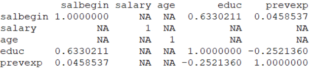
As we can see, there are some issues with the matrix. Firstly, the coefficients themselves have an unnecessary number of decimal places, and secondly, the default settings mean that any columns containing missing values (such as salary or age) generate NA values in the matrix. Therefore, it makes sense to wrap the procedure using a round(,)function, which in this case, rounds the coefficients to two decimals places. We can also add the argument use = “pairwise.complete.obs” within the cor procedure itself, so that the coefficients are based on valid pairwise values (this is the equivalent of the Exclude Cases Pairwise option in SPSS Statistics). As a result, our code now looks like the following.
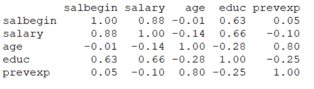
CORRmat <- round(cor(df_CORR, use = "pairwise.complete.obs", ),2)To see a preview of this corrected correlation matrix, we can run the head(CORRmat) procedure which generates the following output.
Having created a satisfactory correlation matrix in the file CORRmat, we can execute the procedure ggcorrplot(CORRmat)to display it as a correlogram using the ggcorrplot package’s default settings.
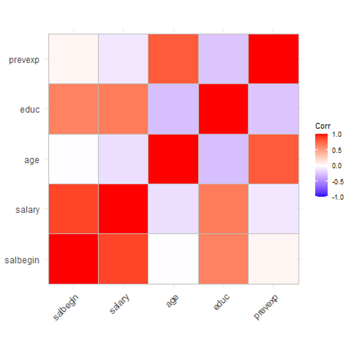
Note that the default correlogram output doesn’t label the correlation cells and shows the full matrix of interactions between each pair of variables. Having established how to create a correlation matrix and how to use the ggcorrplot package to generate this output, we can take a deeper look at the package’s functionality to see how we can include additional arguments to include coefficient labels and control different aspects of the appearance of the correlogram. Consider the following snippet which concerns only the code related to the ggcorrplot() command.
ggcorrplot(CORRmat,
type= "lower",
outline.color = "black",
lab = TRUE,
lab_size = 5,
hc.order = FALSE,
ggtheme = ggplot2::theme_gray,
colors = c("#6D9EC1", "white", "#E46726"))
The first thing to notice is that within the procedure’s main parentheses ( ) there are a number of additional (optional) arguments with each one separated by a single comma.
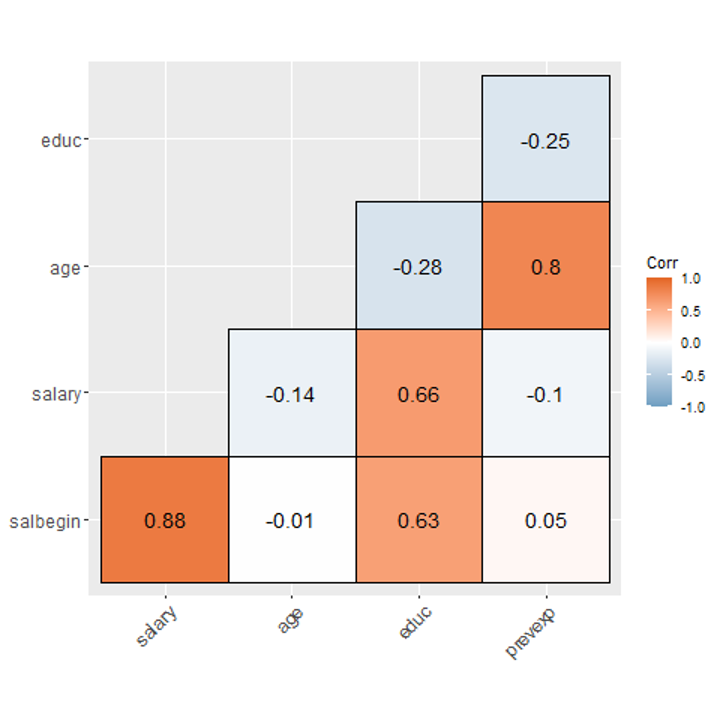
The argument type= “lower” requests that the lower half of the correlation matrix is displayed. The three optional elements for this particular argument are “full”, “lower” and “upper”.
The outline.color = “black” option controls the colour of the lines around the outside of each coefficient cell.
The option lab = TRUE simply requests that the cells in the matrix display the correlation coefficient values contained in the data frame CORRmat. The default for this option is FALSE. The lab_size = 5 setting allows the user to control the display size of these labels.
Next, we have a switch that allows us to cluster the coefficients within the correlogram. If the option hc.order equals TRUE then the coefficients will grouped using a hierarchical cluster function.
The background theme of the correlogram is controlled via the following statement ggtheme = ggplot2::theme_gray. This part of the code refers to the package ggplot2. This is a popular R package based on “The Grammar of Graphics“. The default value is theme_minimal. Other allowed values include theme_gray, theme_light, theme_dark, theme_bw, theme_minimal and theme_classic. If for any reason the ggplot2 package has not already been installed, users can of course add an install.packages(“ggplot2”)near the start of the overall code block.
Finally, we have options for controlling the three colours that constitute the correlogram’s shading. The line colors = c(“#6D9EC1”, “white”, “#E46726”))can be edited to change the colours for negative, neutral and positive correlations respectively. In this example, the negative and positive colours are denoted using hex colour codes. Thankfully, it’s fairly easy to discover what particular colour a hex code refers to by simply pasting the value into a search engine. For example, a Google search of the hex code #6D9EC1 produces the following result.
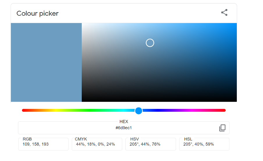
We can then use the colour picker in the search results to choose a new colour before copying and pasting its associated hex code back into our syntax.
It should be pointed out that the ggcorrplot R package includes a lot of other optional elements that we haven’t touched on, but you can find out more about these additional controls here.
Having edited the correlogram code, our full syntax code block now looks like this:
BEGIN PROGRAM R.
#install.packages("ggcorrplot")
library (ggcorrplot)
df_SPSS <- spssdata.GetDataFromSPSS()
df_CORR <- df_SPSS[c('salbegin','salary','age','educ','prevexp')]
CORRmat <- round(cor(df_CORR,  use = "pairwise.complete.obs", ),2)
ggcorrplot(CORRmat,
type= "lower",
outline.color = "black",
lab = TRUE,
lab_size = 5,
hc.order = FALSE,
ggtheme = ggplot2::theme_gray,
colors = c("#6D9EC1", "white", "#E46726"))
END PROGRAM.
The resultant correlogram now appears as:
In the next blog post, we will look at how we can use the Custom Dialog Builder in IBM SPSS Statistics v29 to create our own customised correlogram SPSS dialog by incorporating our R code.