In this series of ‘eat your greens‘ posts looking at core statistical concepts in more detail, we have looked closely at what a test of statistical significance actually is. In particular, we have focused on how to interpret the statistical probability value that various tests generate. This value, often labelled ‘P=’, ‘Prob’ or ‘Sig.’ in stats packages like SPSS, shows the probability of getting a result as extreme as the one observed, assuming the null hypothesis is true. Moreover, students of statistics are taught to reject the null hypothesis if this probability falls below a pre-specified value (e.g. P= 0.05) on the basis that this indicates the evidence does not support the null hypothesis.
However, we must be mindful that even if the ‘P’ value is quite small, it is not impossible that the null hypothesis is in reality true. In fact, there are plenty of examples of researchers rejecting null hypotheses on the basis of ‘P’ values only to find that subsequent follow-up studies can find no evidence to justify this (for more information see the Replication Crisis). This kind of mistake, where a null hypothesis is rejected despite being true, is known as a Type 1 Error. As you can imagine, it’s also possible that one might accept a null hypothesis when in fact it should have been rejected, in which case a Type 2 Error has occurred.
You may already be aware that, when running a statistical test, depending on the context in which they are working, some researchers pre-specify the probability threshold below which the null hypothesis should be rejected at 0.05 (i.e. 5%), whereas as other researchers may set this threshold at 0.01 (1%). This is known as the size of a test and the threshold value itself is called alpha. In fact, it alpha indicates the probability of a Type 1 Error occurring, assuming that the null hypothesis is true. Furthermore, just as researchers should pre-specify the probability threshold of a Type 1 Error before conducting a test, they are also able to pre-specify the probability threshold of a Type 2 Error occurring assuming the alternative hypothesis is true. This threshold value is known as the beta level.
In practice, researchers normally work with a value based on 1-beta which they refer to as the power of a test. The power of a test indicates the probability of rejecting a null hypothesis in favour of the alternative hypothesis when the alternative hypothesis is actually true. In simple terms, it shows the likelihood of your test finding an effect or relationship when it really does exist in the population. The convention is, that most researchers aim for a test which has an 80% chance of detecting an effect if one exists (i.e. Power = 0.8).
But we should be aware that both the size and the power of statistical tests are greatly affected by factors like sample size. If we can’t change the sample size, then it follows that making the alpha level smaller means that the test may be less powerful, and we may be in danger of committing a Type 2 Error. Conversely to make the test more powerful, we may need to sacrifice our strict alpha level value and in doing so, increase the chance of a Type 1 Error occurring.
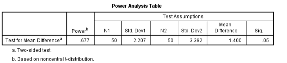
SPSS Statistics now includes Power Analysis calculation procedures that enable users to estimate the necessary sample sizes to achieve the desired threshold values for a test’s size and power. The next table shows the results from a power analysis where the researcher was interested in comparing the performance of male and female subjects in an observation skills experiment. A previous research paper showed that women scored 15.78 (with a standard deviation of 2.21) and men scored 14.38 (with a standard deviation of 3.39). Assuming we got the same results, if the researcher sets alpha at 0.05, how powerful would a t-test be if it were comprised of two groups of 50 men and 50 women? Unfortunately, the results indicate that the t-test would yield a power of 0.677 which is below the desired threshold of 0.8.
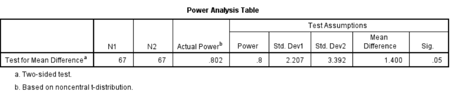
The researcher is nevertheless able to repeat the analysis, but this time they request that the procedure calculates how many cases are required to achieve a power value of 0.8. As the next output table shows, the procedure indicates that they would need a sample size of 67 men and women each (columns N1 and N2) to meet the desired threshold of statistical power.