Earlier in this series of ‘eat your greens‘ postings I looked at the issue of declaring something to be ‘statistically significant’. The purpose of that post was to highlight the fact that not all statistical results are worthy of being regarded as ‘eureka!’ moments just because the findings are unlikely to have occurred due to chance. I’ve also explored the pitfalls of regarding statistical procedures as tests rather than as calculations designed to make an inference.
In this post, I thought it would be useful to look at a worked example in order to explore the context and interpretation of a classic inferential statistical procedure: the independent samples t-test.
A t-test is a statistical procedurethat is commonly employed when an analyst wishes to compare two mean values. The t-test was developed by WS Gosset who was employed as Head Experimental Brewer for Guinness in the early 20th Century. Publishing under the pseudonym ‘Student’, Gossett proposed a method based on the t distribution that could be used to help estimate a mean value within a normally distributed population (i.e. a mean parameter) when the sample size was relatively small. The independent samples t-test is so called because it is used to compare two separate groups in a dataset (such as two different regions). Conversely the related samples t-test is commonly used to compare the mean scores of the same group over time – such as before and after a treatment has been administered.
With any inferential ‘test’, it’s vital that the analyst understands the null hypothesis associated with the procedure. In a t-test remember, two mean values are being compared. Moreover, given that they are unlikely to be exactly the same, we might ask are they different from one another because of random chance, or because the sample that they are drawn from simply reflects the fact that they are different in the population?
With this in mind, the t-test can be used to address the null hypothesis that the two means are equal in the population. As an example, the table below shows the mean number of days spent in hospital by those who are deemed to be ‘Physically Active’ (5.25) compared to those that are categorised as not ‘Physically Active’ (5.55).
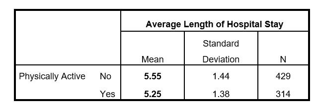
Bear in mind that this difference is quite small: a mere 0.3 days. Nevertheless, with standard deviations of around 1.4 days and over 300 cases in both groups, someone might reasonably ask if this difference is so small that the mean number of days is in reality the same value in population. In which case, they could argue that there is not enough evidence to conclude that being physically active has any bearing on the average length of hospitalisation for patients.
In a previous post I introduced the notion of a standard-error statistic. In that example, we looked at how the standard error could be used to estimate the ‘reliability’ of a sample mean. In the next table, we see the results of a t-test procedure to compare our two group means. Notice that the last column is refers the standard error of the difference. This reveals that a key component of a t-test is an estimate of the reliability of the difference in the two means.
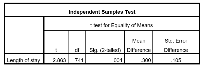
We can also see that the column labelled ‘Sig. (2-tailed)’ shows a probability value of 0.004 (or 0.4%). The ‘2-tailed’ label simply indicates that the test is ignoring whether the difference between the groups is negative or positive (i.e. we make no assumptions as to whether being physically active increases or decreases the mean number of days in hospital). So how should this result be interpreted against our null hypothesis?
The first thing to understand is, that in spite of what many of us are taught, this value is not the ‘probability that the null hypothesis is true’. Significance (or ‘P’) values are focussed on the data (or the ‘evidence’), not the hypothesis. In this case, ‘the data’ refers to the t value which has been calculated by dividing the difference between the two means (0.3) by the Standard Error of the Difference (0.105). Larger t values yield smaller significance (or ‘P’) values. In significance tests, results labelled ‘Sig. (2-Tailed)’ or ‘Prob=’ show the probability of getting a result as ‘extreme’ as our t statistic (or whichever distributional value the relevant procedure uses), assuming that the null hypothesis is true.
As the t statisticis really an expression of the difference in the two means when we take into consideration the standard deviations and the sample sizes, what we can say, is that we would only see a difference as ‘extreme’ as this (0.3 days) in comparable samples around 0.4% of the time, assuming that in reality the average length of stay is same for both groups in the population.
However, we need to bear in mind that as we are dealing with two groups of fairly large samples and relatively small measures of variation (the standard deviations). So it is perhaps not surprising that even a small difference in the mean values yields a small probability value. In other words, it’s easy to generate a ‘significant’ result if the data are strong even when the effect is not.