Take a look at the table below. It describes a relatively common situation in business analytics. Two offers have been made to a sample of 40,000 prospective readers of a magazine. As an experiment, half of the prospects have been offered a 25% discount for the first year and the other half have been offered an extended subscription of 15 months (rather than the normal 12 months).
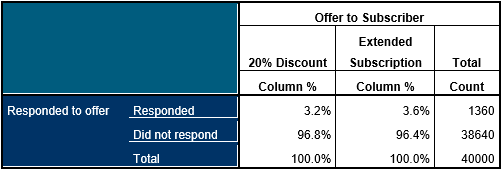
The table seems to indicate a slight increase in the response rate (a mere 0.4%) for those offered the extended subscription. The business analysts want to know how probable it is that this is simply a random effect or whether the extended subscription is indeed more likely to elicit a response. If by this stage you are thinking that a tiny difference of 0.4% really isn’t worth bothering about, you might want to consult this article.
In modern parlance, this type of problem is commonly referred to as A/B testing but in reality the methods used to address it are over 100 years old. One such approach is apply a test of statistical significance such as the Pearson Chi Squared test. Generally speaking, tests like chi-squared are used to examine differences with between fields with different categories.
Without getting too deep into the technicalities of how it is calculated, the Chi squared value is derived by comparing the frequency values (count) that we observe in a table and the expected frequencies that we would expect to see if there was no bias towards one group or another. If we flip a coin a 100 times and the outcome is 54 ‘heads’ and 46 ‘tails’ we may not instinctively be able to calculate the probability that the coin is biased but we know that if it wasn’t biased, on average we should see a 50/50 outcome: this represents our expected frequency.
Let’s look at the table again, but this time we can compare the observed and the expected frequencies (which are shown in red).
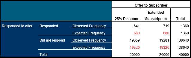
We can see that the 25% discount offer elicited 39 fewer responses than would be expected if both offers had the same effect (whereas the exact opposite is true of the extended subscription offer). The Chi-Squared calculation sums these differences between the observed and expected counts and then (with a few adjustments depending on the method used) calculates the probability that the differences we have observed in the table are the result of random chance rather than a real effect that is likely to exist in the population of all potential magazine subscribers. In other words, it indicates whether the extended subscription offer is likely to be more tempting to prospects than the 25% discount offer. The table below shows the results of the Chi-Squared test.
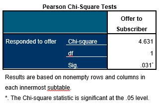
The value that we need to focus on is in the row marked ‘Sig.’. This is an estimate of probability. In this instance, a probability value of 0.031 indicates that the differences between the groups are sufficiently large that we would only expect to observe this 3.1% of the time randomly. In short, the difference between the response rates for the two offers is not very likely to be the result of mere chance.
So how small does the probability have to be before you come to this conclusion? Well, that depends on the context of the analysis, but generally a value less than 0.05 (or 5%) is regarded as small enough to be viewed as ‘statistically significant’. In this case the business analysts could conclude that there is good evidence to suggest that the extended subscription offer is likely to yield slightly more customers than offering a 25% discount.